NanoVer Basics
This page is a great starting point for those who are new to NanoVer. Make sure that you have already installed NanoVer, so that you can use the information on this page to start running interactive molecular dynamics (iMD) simulations with NanoVer.
Jupyter notebook tutorials
We provide a set of short Jupyter notebook tutorials that introduce NanoVer as a framework for running interactive molecular dynamics simulations. These notebooks are designed to provide new users with some basic examples that demonstrate how to get up and running with NanoVer, and exhibit some core features of NanoVer in a quick, intuitive way. If you are new to NanoVer, these tutorials are the perfect place to start!
Here we give a summary of the available Jupyter notebook tutorials, that can be found in the tutorials folder of the GitHub repository:
getting_started: New to NanoVer? Start here! An introductory notebook that showcases how NanoVer can be used to run an interactive molecular dynamics (iMD) simulation for a pre-prepared methane & nanotube system.
recording_and_replaying: An introductory notebook that demonstrates how NanoVer can be used to record and replay iMD simulations.
multiple_simulations: This notebook demonstrates how to load and run multiple simulation files using a single OmniRunner server, providing default visualizations, and details how to switch between them using the Jupyter notebook and XR interfaces.
nanover_nglview: A notebook that assumes a server is already running, and visualises it with NGLView.
runner_GUI: A notebook that demonstrates how to use the NanoVer GUI to run a server.
Running a server
The NanoVer Python server
The NanoVer Python Server package can be installed using conda (see User Installation Guide) or using the source code (see Developer Installation Guide). Once installed, you can run a NanoVer server using either (a) a Python script or Jupyter notebook or (b) the command line.
via a Python script or Jupyter notebook
For running a NanoVer server using a Python script or Jupyter notebook, please see our Tutorials page. If you are new to NanoVer, we recommend starting with our getting_started notebook.
via the command line
Once you have the nanover-server package installed in your conda environment, you will be able to use the
nanover-server command to run a server.
This server can take any of the following:
A NanoVer OpenMM simulation
A NanoVer OpenMM simulation with ASE as an interface
A NanoVer recording, with either or both of the trajectory and shared state recording files
Note that you can give the simulations/recordings either explicitly as a string or simply by typing the file path. Here are some example commands:
# load a single NanoVer OpenMM simulation
nanover-server --omm "my-openmm-sim.xml"

# load multiple simulations
nanover-server --omm "my-openmm-sim-1.xml" "my-openmm-sim-2.xml" --omm-ase "my-ase-omm-sim.xml"

# load a NanoVer recording
nanover-server --playback "my-recording.state" "my-recording.traj"
For more information about the arguments provided with this command, type:
nanover-server --help
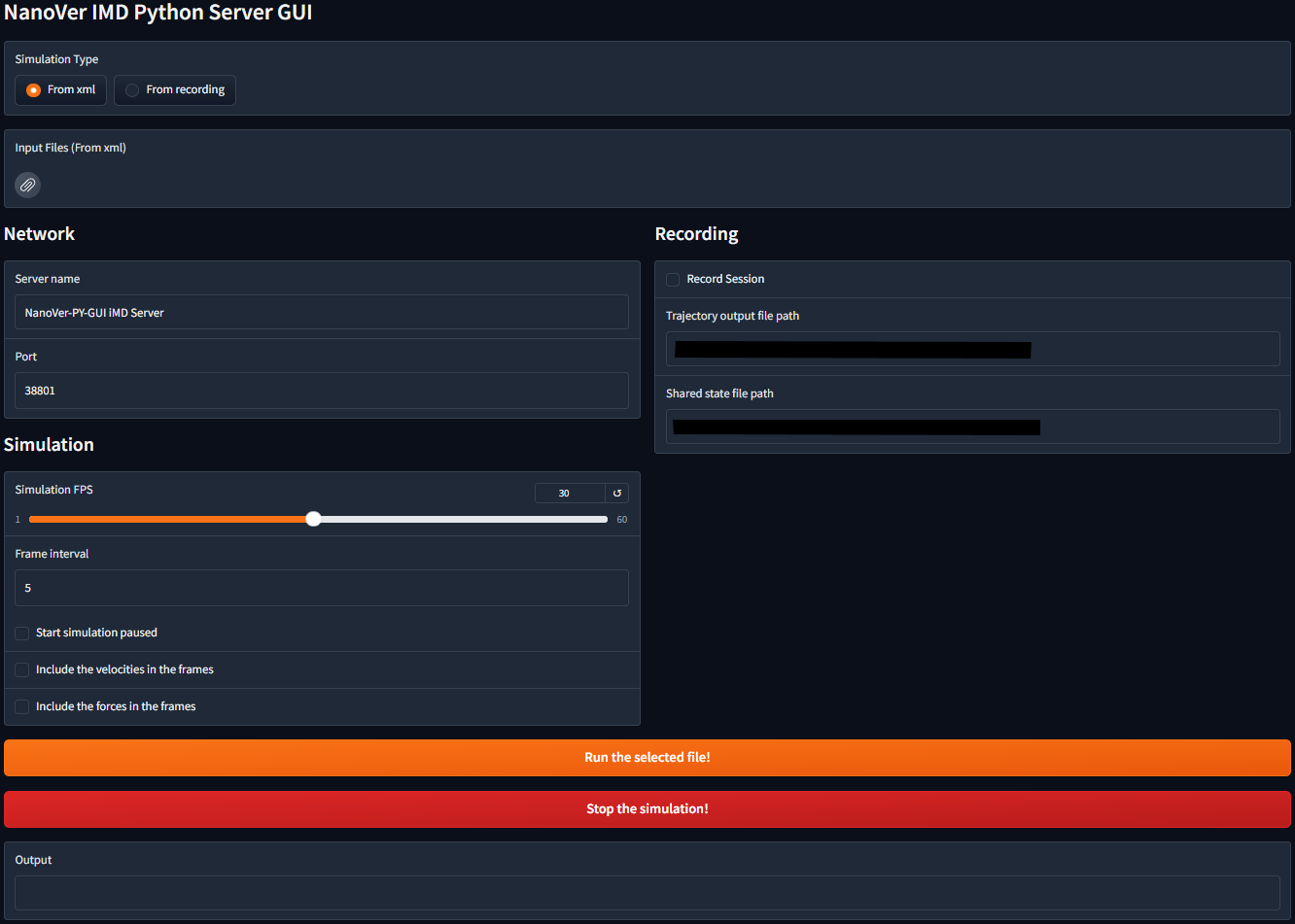
via the GUI
The Python GUI creates a web-based graphical interface for running a NanoVer Server. It supports both real-time simulations from NanoVer OpenMM XML files and playback of recorded trajectories. The interface provides controls for simulation parameters, network settings, and trajectory recording options.
To run a server via the GUI there are two options:
Open the
runner_GUI.ipynbnotebook where you will find a step by step guide on how to use the GUI.Run the GUI directly from the command line by running
UI.py.
If everything is set up correctly, you should see the following interface:
Recording a session
For a NanoVer session to be useful beyond the time spent in XR, we want to record it! We can then use this recording to run our analysis, or replay it to get insight. In this section, we describe how to record a NanoVer session and how to visualise the recording using inbuilt NanoVer methods.
If you would like to know more about the format of NanoVer recordings, please go to the recording in NanoVer Concepts page.
Recording with Python
via the terminal
The nanover-record command-line utility can be used to quickly start and stop multiple spans of recording without writing any code.
The default is to connect to a local server on the default port, but more connectivity and output options can be found with the help option:
nanover-record --help
via a Python script
NanoVer sessions can be also recorded using the nanover.websocket.record module.
Here is an example of how to define the file names and paths for the recording and pass them to the recording function:
from nanover.websocket.record import record_from_server
# Define the file names path
recording_path = 'path/to/simulation_recording.nanover.zip'
# create a recording from a server and save it to the files
record_from_server("ws://localhost:38801", recording_path)
Visualising recordings
Visualising and playing back recordings can be done using nanover.recording module.
The Python Server can stream recorded NanoVer streams read by a PlaybackSimulation object to a client.
The client then plays back the recording as if it were a live stream.
The server sends the frame and state updates whilst trying to respect the timing dictated by the timestamps stored
in the file.
from nanover.app import OmniRunner
from nanover.recording import PlaybackSimulation
simulation_recording = PlaybackSimulation.from_path('path/to/recording.nanover.zip', name='simulation-recording')
# Create a runner for the simulation
recording_runner = OmniRunner.with_basic_server(simulation_recording,
                                                name='simulation-recording-server')
# Start the runner
recording_runner.next()
# Close the runner
recording_runner.close()
Note
Further instructions and information on how to record and replay using the NanoVer Python module can be found in this notebook recording_and_replaying.ipynb.
Processing NanoVer recordings
With NanoVer and MDAnalysis
Recordings can be read and manipulated using the NanoVer Python library.
The nanover.mdanalysis module enables us to convert NanoVer trajectory recordings into
MDAnalysis Universes, which are data structures
used by the MDAnalysis library to handle molecular dynamics simulations.
A single NanoVer recording may include switching between multiple systems with differing topologies, whereas a single MDAnalysis universe is concerned only with single systems of constant topology. NanoVer provides a universes_from_recording function to extract each independent simulation run within a single NanoVer trajectory recording.
See the example code below, or check out the mdanalysis_nanover_recording Jupyter notebook tutorial for further information.
import MDAnalysis as mda
from nanover.mdanalysis import universes_from_recording
import matplotlib.pyplot as plt

# read all universes and take the first one
universes = universes_from_recording(traj='hello.traj')
u = universes[0]

times = []
frames = []
potential_energy = []
kinetic_energy = []
user_energy = []
timestamps = []

for timestep in u.trajectory:
    frames.append(timestep.frame)
    times.append(timestep.time)
    potential_energy.append(timestep.data["energy.potential"])
    kinetic_energy.append(timestep.data["energy.kinetic"])
    user_energy.append(timestep.data["energy.user.total"])
    timestamps.append(timestep.data["elapsed"])

fig, axis = plt.subplots(1)
axis.plot(frames, potential_energy, label='Potential energy')
axis.plot(frames, kinetic_energy, label='Kinetic energy')
axis.plot(frames, user_energy, label='User energy')
axis.legend()
axis.set_ylim(-1000, 10000)
axis.set_xlabel("Frame index")
axis.set_ylabel("Energy (kJ/mol)")